Table of Contents
Stochastic Gradient Descent (v.2)
Learning algorithms based on Stochastic Gradient approximations are known for their poor performance on optimization tasks and their extremely good performance on machine learning tasks (Bottou and Bousquet, 2008). Despite these proven capabilities, there were lingering concerns about the difficulty of setting the adaptation gains and achieving robust performance. Stochastic gradient algorithms have been historically associated with back-propagation algorithms in multilayer neural networks, which can be very challenging non-convex problems. Stochastic gradient algorithms are also notoriously hard to debug because they often appear to somehow work despite the bugs. Experimenters are then led to believe, incorrectly, that the algorithm itself is flawed.
Therefore it is useful to see how Stochastic Gradient Descent performs on simple linear and convex problems such as linear Support Vector Machines (SVMs) or Conditional Random Fields (CRFs). This page proposes simple code examples illustrating the good properties of stochastic gradient descent algorithms. The provided source code values clarity over speed.
- The first release of this code (2007) was written to accompany my 2007 NIPS tutorial on large scale learning.
- The second major release of this code (2011) adds a robust implementation of the averaged stochastic gradient descent algorithm (Ruppert, 1988) which consists of performing stochastic gradient descent iterations and simultaneously averaging the parameter vectors over time. When the stochastic gradient gains decrease with an appropriately slow schedule, Polyak and Juditsky (1992) have shown that the convergence is asymptotically as efficient as second-order stochastic gradient descent with much smaller computational costs. One can therefore hope to match the batch optimization performance after a single pass on the randomly shuffled training set (Fabian, 1978; Bottou and LeCun, 2004). Achieving one-pass learning in practice remains difficult because one often needs more than one pass to simply reach this favorable asymptotic regime. The gain schedule has a deep impact on this convergence. Finer analyses (Xu, 2010; Bach and Moulines, 2011) reveal useful guidelines to set these learning rates. Xu (2010) also describe a wonderful way to efficiently perform the averaging operation when the training data is sparse. On problems with moderate dimension, the resulting algorithm reaches near-optimal test set performance in one or two passes. When the dimension increases, the advantage erodes, but the algorithm remains competitive.
Download and Compilation
Downloading the programs
- Create a clone of the git repository with command:
git clone http://leon.bottou.org/git/sgd.git
- As an alternative, you can still download the tarball sgd-2.1.tar.gz released in September 2012. This is no longer the recommended approach but should still work.
- Make sure to read the files
“README.txt”and“data/README.txt”.
Downloading the datasets
- Download the following files from the RCV1-V2 web site and install them in directory
“data/rcv1”.
- Download the following files from the Pascal Large-Scale Challenge server and install them in directory
“data/pascal”.- Optionally, webspam_train.lab.bz2, webspam_train.dat.bz2 (1.5GB)
- Download the following files from the CONLL2000 Chunking web site and install them in directory
“data/conll2000”.
- Run the conversion script for the Pascal datasets. This requires Python and takes some time.
   $ cd data/pascal
   $ ./convert.py -o alpha.txt alpha train
   $ ./convert.py -o webspam.txt webspam train    # (optional)
Compiling
- To compile under Linux, simply type
“make”in the toplevel directory. The compilation requires the ZLib library. Most Linux distributions provide this by default. Things should be very similar under other Unix operating systems. - To compile under Windows, see the file
“win/README.txt”.
Stochastic Gradient SVM
The SVM programs are located in directory “sgd/svm”.
The file “svm/README.txt” provides the full details and describes how to run various experiments.
SvmSgd
Program “svmsgd” implements a straightforward stochastic gradient descent algorithm.
- The learning rate has the form η0 / (1 + λ η0 t) where λ is the regularization constant.
- The constant η0 is determined by performing preliminary experiments on a data subsample.
- The learning rate for the bias is multiplied by 0.01 because this frequently improves the condition number.
- The weights are represented as the product of a scalar and a vector in order to easily implement the weight decay operation that results from the regularization term.
Points (1) and (4) follow (Shalev-Schwartz et al., 2007).
SvmAsgd
Program “svmasgd” implements the averaged stochastic gradient descent algorithm.
- The learning rate has the form η0 / (1 + λ η0 t) 0.75 where λ is the regularization constant.
- The constant η0 is determined by performing preliminary experiments on a data subsample.
- Averaging starts only at the second epoch. The first epoch is a simple stochastic gradient descent. This provides more robust convergence at the expense of one additional epoch. You can use option
-avgstartto change this. - Both the stochastic gradient weights and the averaged weights are represented using a linear transformation that yields efficiency gains for sparse training data.
Points (1) and (4) follow (Xu, 2010).
RCV1 Benchmark
The benchmark task is the recognition of RCV1 documents belonging to the class CCAT.
Program “prep_rcv1” reads the RCV1-V2 token files from directory “data/rcv1” and computes the TF/IDF features on the basis of the our training set. This programs produces the two files “rcv1.train.bin.gz” and “rcv1.test.bin.gz” containing our training and testing sets. This short program also generates files in SvmLight format when compiled with option -DPREP_SVMLIGHT.
| Benchmark | Features | Training examples | Testing examples |
|---|---|---|---|
| RCV1 | 47152 | 781265 | 23149 |
| Algorithm (hinge loss, λ=1e-4) | Training Time* | Primal cost | Test Error |
|---|---|---|---|
| SMO (SVMLight) | ≃ 16000 secs1 | 0.2275 | 6.02% |
| Cutting Plane (SVMPerf) | ≃ 45 secs2 | 0.2278 | 6.03% |
| Hinge Loss SDCA (LibLinear -s 3 -B 1) | 2.5 secs | - | 6.02% |
SGD (svmsgd) | < 1 sec. | 0.2275 | 6.02% |
ASGD (svmasgd) | < 1 sec. | 0.2275 | 6.02% |
1 Extrapolated from a 23642 seconds run on a 30% slower machine.
2 Extrapolated from a 66 seconds run on a 30% slower machine.
* All timings exclude data loading time.
| Algorithm (log loss, λ=5e-7) | Training Time | Primal cost | Test Error |
|---|---|---|---|
| TRON (LibLinear -s 0 -B 1) | 33 secs | - | 5.14% |
| SDCA (LibLinear -s 7 -B 1) | 15 secs | - | 5.13% |
SGD (svmsgd) | 4 secs | 0.1283 | 5.14% |
ASGD (svmasgd) | 5 secs | 0.1281 | 5.13% |
Alpha Benchmark
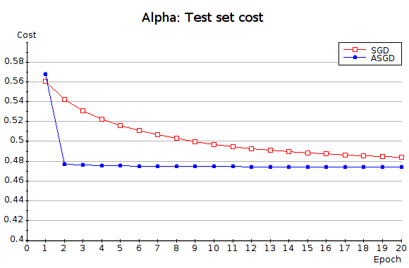
You must first convert the original Pascal files using the Python script convert.py as explained above. Program “prep_alpha” then reads the converted Pascal file “data/pascal/alpha.txt” and produces the two files “rcv1.train.bin.gz” and “rcv1.test.bin.gz” containing our training and testing sets. The alpha dataset illustrates how ASGD sometimes vastly outperforms plain SGD. The plot below shows how ASGD reaches near-optimal test performance only one pass after the activation of the averaging code (epoch 2.)
| Benchmark | Features | Training examples | Testing examples |
|---|---|---|---|
| Alpha | 500 | 250000 | 250000 |
| Algorithm (log loss, λ=1e-6) | Training Time | Primal cost | Test Error |
|---|---|---|---|
| TRON (LibLinear -s 0 -B 1) | 115 secs | - | 21.86% |
| SDCA (LibLinear -s 7 -B 1) | 19 secs | - | 21.86% |
SGD (svmsgd) | 51 secs | 0.4717 | 21.95% |
ASGD (svmasgd) | 4 secs | 0.4713 | 21.86% |
Stochastic Gradient CRFs
The CRF programs “crfsgd” and “crfasgd” respectively use the SGD and ASGD algorithms
to train a Conditional Random Field. The algorithms
are setup exactly as the SVM variants, but the implementation accounts for
the greater structural complexity of conditional random fields.
Both programs accept the same input files as the well known
CRF++ software by Taku Kudo.
They produce the same tagging files which can be analyzed using the CONLL perl script “conlleval”.
They use the same template files to specify the features and accept the same data files.
For convenience, “crfsgd” and “crfasgd” can also directly read gzipped data files.
See the CRF++ documentation for details.
CONLL 2000 Benchmark
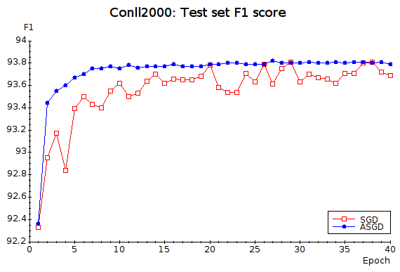
Our CRF benchmark is the CONLL2000 Text Chunking task, which consists of dividing a text in syntactically correlated segments (noun phrases, verb phrases, etc.). We use the feature template that comes with CRF++.
| Benchmark | Parameters | Training sentences | Training chunks | Testing sentences | Testing chunks |
|---|---|---|---|---|---|
| CONLL2000 | 1679700 | 8936 | 106978 | 2012 | 23852 |
| Algorithm (-f 3 -c 1) | Training Time | Primal cost | Test F1 score |
|---|---|---|---|
| LBFGS (CRF++) | ≃ 3000 secs3 | 9042 | 93.74% |
SGD (crfsgd) | 303 secs | 9096 | 93.73% |
ASGD (crfasgd) | 134 secs | 9204 | 93.79% |
3 Extrapolated from a 4335 seconds run on a 30% slower machine.
References
pdf.
Changelog
| Version | Date | Comments |
|---|---|---|
| sgd-1.0.tar.gz | 2007-08-22 | Initial release. |
| sgd-1.1.tar.gz | 2007-10-04 | Relicensed under LGPL |
| sgd-1.2.tar.gz | 2008-04-07 | Bug fix in svm/reprocess.cpp. Thanks to Wei Xu. |
| sgd-1.3.tar.gz | 2009-01-31 | Added SSE2 code for dense vectors. |
| sgd-2.0.tar.gz | 2011-10-12 | Major release featuring sgd and asgd. |
| sgd-2.1.tar.gz | 2012-09-14 | Bug fix: istream::unget() does not clear eof bit |
| Latest | git clone http:leon.bottou.org/git/sgd.git |
|
Related projects
Rather than emphasizing performance or generality, this code favors readability. I am therefore glad to see that many authors of machine learning projects have found it useful, sometimes directly, sometimes as a source of inspiration. Here are a few links:
- Implicit SGD uses the SVMSGD code as a starting point.
- SciKit contains a SGD optimizer inspired by SVMSGD.
- Shogun contains a SGD module derived from SVMSGD.
- …


