Table of Contents
Fast Kernel Classifiers with Online and Active Learning
Abstract: Very high dimensional learning systems become theoretically possible when training examples are abundant. The computing cost then becomes the limiting factor. Any efficient learning algorithm should at least pay a brief look at each example. But should all examples be given equal attention? This contribution proposes an empirical answer. We first presents an online SVM algorithm based on this premise. LASVM yields competitive misclassification rates after a single pass over the training examples, outspeeding state-of-the-art SVM solvers. Then we show how active example selection can yield faster training, higher accuracies, and simpler models, using only a fraction of the training example labels.
Remark: The appendix proposes very general theorems for the convergence of direction search algorithms for convex optimization. This applies to SMO and to many of its variants such as the algorithms discussed in this paper. See the erratum below.
@article{bordes-ertekin-weston-bottou-2005,
  author = {Bordes, Antoine and Ertekin, Seyda and Weston, Jason and Bottou, L\'{e}on},
  title = {Fast Kernel Classifiers with Online and Active Learning},
  journal = {Journal of Machine Learning Research},
  year = {2005},
  volume = {6},
  pages = {1579-1619},
  month = {September},
  url = {http://leon.bottou.org/papers/bordes-ertekin-weston-bottou-2005},
}
1. Implementation
The complete source code is available on the LaSVM project page.
2. Data Sets
The following datasets were used for experiments
| File | Description |
|---|---|
| lasvm-adult.tar.bz2 | The “Adult” dataset |
| lasvm-banana.tar.bz2 | The “Banana” dataset |
| lasvm-postal.tar.bz2 | The “USPS” and “USPS+N” datasets |
| lasvm-reuters.tar.bz2 | The “Reuters/MoneyFX” dataset |
| lasvm-waveform.tar.bz2 | The “Waveform” dataset |
| lasvm-mnist.tar.bz2 | The “MNIST” dataset (see note 1) |
| lasvm-forest.tar.bz2 | The “Forest” dataset (a.k.a. “Covertype”, see note 1) |
Note 1
Experimental results reported for the MNIST and Forest datasets were obtained by interfacing both the LIBSVM and LASVM code with Lush. The corresponding code can be found in the Lush repository. This arrangement has allowed us to benefit from optimized fast kernels implemented in Lush.
- File
mnist.tar.bz2contains data files suitable for use by thela_svmandla_testprograms. See theREADMEfile for details.
- File
forest.tar.bz2does not contain data files suitable for use by thela_svmandla_testprograms. It contains a C file with the specialized kernel implementation. See theREADMEfile for details.
Note 2
We observed little variations of the recognition accuracies from one platform to the next. We believe these variations are caused by different implementations of the rand() function, and by different rounding of floating point values.
3. Complement
An anonymous reviewer (for another paper) suggested that similar results might be achieved by manipulating the stopping criterion of the SMO algorithm. Although such an early stopping technique is known to be difficult to tune, the suggestion deserves attention. The LIBSVM stopping criterion is controlled by the ε parameter. The test set performance hardly depends on this parameter as long as it is small enough. The performance degrades abruptly when ε exceeds a problem dependent critical value.
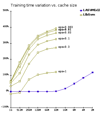
We carried out experiments using the MNIST dataset. Figure 6bis above is comparable to Figure 6 in the paper. The horizontal axis displays various kernel cache sizes. The vertical axis reports the training time variations relative to LIBSVM with a one gigabyte kernel cache. These changes are averaged over the ten MNIST classifiers. The blue curve shows the LASVM times. The yellow curves show the LIBSVM times with early stopping using various values of the ε parameter. The highest value ε=1 represents the first value of ε for which we could measure a reliable loss of accuracy on the test set. For this particular problem, LIBSVM performs as fast as LASVM when ε is chosen optimally and when the kernel cache is very large. LASVM remains much more efficient when the memory is constrained.
4. Erratum
In the appendix, section A.1, notations, the definition of ƒ* should specify that λ remains positive, as shown below:
\[ \begin{array}{rcl} \Phi(x,u) & = & \max\left\{ \lambda\ge0 ~|~ x+\lambda u \in {\cal F} \right\} \\ f^*(x,u) & = & \max\left\{ f(x+\lambda u) ~|~ x+\lambda u \in {\cal F},~ \lambda\ge0 \right\} \end{array} \]
5. See also
- The LASVM software.
- A book chapter where we describe a SVM trained with 8 million examples on a single processor using LASVM.
